Sample Inspector (Part II)
Contents
Sample Inspector (Part II)
This notebook compares the Microsoft Digitised Books collection to the genre annotations. We’d like to know if the annotated sample deviates from the digital collection and look at aspects that should remains stable across both datasets.
%matplotlib inline
import json
import pandas as pd
from collections import Counter
Data processing
First, we load the metadata of the Microsoft Digitised Books collection.
metadata_blb = pd.read_csv(
    "https://bl.iro.bl.uk/downloads/e1be1324-8b1a-4712-96a7-783ac209ddef?locale=en",
    dtype={"BL record ID": "string"},
    parse_dates=False,
)
metadata_blb.head(3)
| BL record ID | Type of resource | Name | Dates associated with name | Type of name | Role | All names | Title | Variant titles | Series title | Number within series | Country of publication | Place of publication | Publisher | Date of publication | Edition | Physical description | Dewey classification | BL shelfmark | Topics | Genre | Languages | Notes | BL record ID for physical resource | |
|---|---|---|---|---|---|---|---|---|---|---|---|---|---|---|---|---|---|---|---|---|---|---|---|---|
| 0 | 014602826 | Monograph | Yearsley, Ann | 1753-1806 | person | NaN | More, Hannah, 1745-1833 [person] ; Yearsley, A... | Poems on several occasions [With a prefatory l... | NaN | NaN | NaN | England | London | NaN | 1786 | Fourth edition MANUSCRIPT note | NaN | NaN | Digital Store 11644.d.32 | NaN | NaN | English | NaN | 3996603 |
| 1 | 014602830 | Monograph | A, T. | NaN | person | NaN | Oldham, John, 1653-1683 [person] ; A, T. [person] | A Satyr against Vertue. (A poem: supposed to b... | NaN | NaN | NaN | England | London | NaN | 1679 | NaN | 15 pages (4°) | NaN | Digital Store 11602.ee.10. (2.) | NaN | NaN | English | NaN | 1143 |
| 2 | 014602831 | Monograph | NaN | NaN | NaN | NaN | NaN | The Aeronaut, a poem; founded almost entirely,... | NaN | NaN | NaN | Ireland | Dublin | Richard Milliken | 1816 | NaN | 17 pages (8°) | NaN | Digital Store 992.i.12. (3.) | Dublin (Ireland) | NaN | English | NaN | 22782 |
Computing the title’s first character.
A simple test for comparing the sample to the Microsoft Digitised Books metadata is computing the probabilities of the title’s first character. This distribution should look similar for both datasets. Below we create a function first_alpha_char that returns the first character of a string. If none could be found, it returns a hashtag.
def first_alpha_char(x):
    """returns the first lowercased alphatical character of a string"""
    try:
        x = x[0].lower()
        x = "".join([c for c in x if c.isalpha()])
        return x[0]
    except:
        return "#"
With .apply() we can extract to first character from the title column.
metadata_blb["first_alpha_char"] = metadata_blb.Title.apply(first_alpha_char)
Next, we use Counter() to count all elements in the first_alpha_char column and turn the counts into probabilities.
char_count = Counter(
    metadata_blb[metadata_blb["first_alpha_char"] != None].first_alpha_char
)
char_probs = {k: v / sum(char_count.values()) for k, v in char_count.items()}
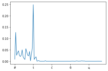
Plotting distribution of first title character
pd.Series(char_probs, index=sorted(char_probs.keys())).plot()
<matplotlib.axes._subplots.AxesSubplot at 0x7fb9a0488f90>
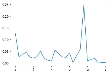
pd.Series(char_probs, index=sorted(char_probs.keys()))["a":"z"].plot()
<matplotlib.axes._subplots.AxesSubplot at 0x7fb997cb64d0>
Next, we apply the same procedure to the annotated sample. We’ll start by loading the annotated sample.
Comparing to the annotated data
annotations = pd.read_csv(
    "https://bl.iro.bl.uk/downloads/36c7cd20-c8a7-4495-acbe-469b9132c6b1?locale=en",
    dtype={"BL record ID": str},
)
annotations.head(1)
/usr/local/lib/python3.7/dist-packages/IPython/core/interactiveshell.py:2718: DtypeWarning: Columns (17,35,37) have mixed types.Specify dtype option on import or set low_memory=False.
  interactivity=interactivity, compiler=compiler, result=result)
| BL record ID | Type of resource | Name | Dates associated with name | Type of name | Role | All names | Title | Variant titles | Series title | Number within series | Country of publication | Place of publication | Publisher | Date of publication | Edition | Physical description | Dewey classification | BL shelfmark | Topics | Genre | Languages | Notes | BL record ID for physical resource | classification_id | user_id | created_at | subject_ids | annotator_date_pub | annotator_normalised_date_pub | annotator_edition_statement | annotator_genre | annotator_FAST_genre_terms | annotator_FAST_subject_terms | annotator_comments | annotator_main_language | annotator_other_languages_summaries | annotator_summaries_language | annotator_translation | annotator_original_language | annotator_publisher | annotator_place_pub | annotator_country | annotator_title | Link to digitised book | annotated | |
|---|---|---|---|---|---|---|---|---|---|---|---|---|---|---|---|---|---|---|---|---|---|---|---|---|---|---|---|---|---|---|---|---|---|---|---|---|---|---|---|---|---|---|---|---|---|---|
| 0 | 014602826 | Monograph | Yearsley, Ann | 1753-1806 | person | NaN | More, Hannah, 1745-1833 [person] ; Yearsley, A... | Poems on several occasions [With a prefatory l... | NaN | NaN | NaN | England | London | NaN | 1786 | Fourth edition MANUSCRIPT note | NaN | NaN | Digital Store 11644.d.32 | NaN | NaN | English | NaN | 3996603 | NaN | NaN | NaN | NaN | NaN | NaN | NaN | NaN | NaN | NaN | NaN | NaN | NaN | NaN | NaN | NaN | NaN | NaN | NaN | NaN | NaN | False |
This dataset includes both annotated data and non-annotated data. Since we only want the annotated data, we can filter these out using the annotated column which contains a flag to indicate if the data has been annotated.
annotations = annotations[annotations["annotated"] == True]
Because of the way in which the annotations were collected we have some duplicates. There are different ways in which we can deal with these duplicates but here we will just drop the duplicates for the Title column.
annotations = annotations.drop_duplicates(subset="Title")
annotations["first_alpha_char"] = annotations.Title.apply(first_alpha_char)
/usr/local/lib/python3.7/dist-packages/ipykernel_launcher.py:1: SettingWithCopyWarning:
A value is trying to be set on a copy of a slice from a DataFrame.
Try using .loc[row_indexer,col_indexer] = value instead

See the caveats in the documentation: https://pandas.pydata.org/pandas-docs/stable/user_guide/indexing.html#returning-a-view-versus-a-copy
  """Entry point for launching an IPython kernel.
char_count_anno = Counter(
    annotations[annotations["first_alpha_char"] != None].first_alpha_char
)
char_probs_anno = {
    k: v / sum(char_count_anno.values()) for k, v in char_count_anno.items()
}
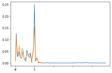
Plotting a comparison between the annotated subset and full collection
pd.Series(char_probs, index=sorted(char_probs.keys())).plot()
pd.Series(char_probs_anno, index=sorted(char_probs_anno.keys())).plot()
<matplotlib.axes._subplots.AxesSubplot at 0x7fb99572a3d0>
annotations["annotator_main_language"].unique()
array([nan, 'lat\nger', 'gmh\nlat\nger', 'ger', 'ger\ngmh\nlat',
       'ger\nfre', 'eng', 'lat\ngmh\nger', 'ger\neng', 'ger\nlat',
       'lat\nfre', 'dut\nfre\nspa', 'fre\nger', 'ger\nfrs\nlat',
       'ger\ngmh', 'lat\ndut\nfrm\nfre', 'ger\nspa', 'eng\nfre'],
      dtype=object)
annotations["english"] = annotations["annotator_main_language"].apply(
    lambda x: str(x).lower().startswith("eng")
)
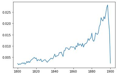
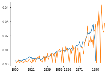
Compare distribution of publication date
Lastly, we can compare the distribution over time to see if the sample is biased towards are certain period.
metadata_blb = metadata_blb[metadata_blb["Date of publication"].notna()].copy(deep=True)
metadata_blb["date"] = metadata_blb["Date of publication"].str.split("-").str[0]
year_counts = Counter(metadata_blb["date"].values)
year_probs = {k: v / sum(year_counts.values()) for k, v in year_counts.items()}
pd.Series(year_probs, index=sorted(year_probs.keys()))["1800":"1900"].plot()
<matplotlib.axes._subplots.AxesSubplot at 0x7fb995d465d0>
year_counts_anno = Counter(annotations["annotator_normalised_date_pub"].values)
year_probs_anno = {
    k: v / sum(year_counts_anno.values()) for k, v in year_counts_anno.items()
}
Below, we made a small function to manipulate the date of publication field by extracting the year (if available) and returning it as an integer.
def get_int(x):
    """return year is integer"""
    try:
        return int(x)
    except:
        pass
    try:
        return int(x.split("-")[0])
    except:
        False


year_probs_anno = {str(k): v for k, v in year_probs_anno.items() if get_int(k)}
Comparing publication dates across the annotated and full collection
pd.Series(year_probs, index=sorted(year_probs.keys()))["1800":"1900"].plot()
pd.Series(year_probs_anno, index=sorted(year_probs_anno.keys()))["1800":"1900"].plot()
<matplotlib.axes._subplots.AxesSubplot at 0x7fb994dad710>
Conclusion
Whilst this wasn’t a super rigorous assessment of the potential differences and similarities between the collections, it does give us some sense of this.
Because we are using our annotated data to train a model that we will then want to use on the whole collection (or at least a more significant part of the collection). We want to be careful about how both of these collections may differ. If there are substantial differences between the two, our model may perform well on our training data but badly on new data. This concept is something we’ll return to frequently in the remaining sections.